One of the most common challenges in a data-driven story is combining two sets of data — such as events and populations — to put a story into context. In an extract from the ebook Finding Stories in Spreadsheets, I explain how to use lookup functions to combine two tables. The longer ebook version of this tutorial includes a dataset and exercise to employ these techniques.

Combining data is often a great way of telling new stories about spreadsheets. For example: you may have one table showing pass rates for each school in an area, and another table showing their addresses. Combining these would allow you to identify geographical patterns, or to place them on a map.

You could also combine the addresses with poverty rates for different locations, or unemployment to see if there’s a possible relationship (remembering that correlation does not equal causation), or to identify the schools performing particularly well despite local conditions. In the video below, for example, I walk through an example of combining data on different sports teams’ attendances with data on their rankings, allowing you to see who’s attracting large crowds despite their poor performance.

The VLOOKUP function is one of the most widely-used tools in combining data in this way. It stands for Vertical lookup, and means that the spreadsheet will look up and down a column (i.e. vertically) for whatever you ask it. In more recent versions of Excel the XLOOKUP function has been introduced to make the process easier — but the process is similar for both.

Prepare the ingredients

If you want to merge information from two tables, you need the following ingredients:

• Two tables containing the data, in the same workbook. It doesn’t matter if they’re on separate sheets, or on one. Unless they’re very small, however, I’d recommend keeping them on separate sheets.
• Each table must have a column in common. It doesn’t have to have the same heading, but it must have the same data. For example, both tables could have a column for institution names, or area, or ID code, postcode, and so on. VLOOKUP and XLOOKUP look for a match between the two tables based on this.
• For VLOOKUP, that column must be to the left of anything you want to grab from a table. So you may need to rearrange your columns a little (XLOOKUP removes this requirement).

Check your data meets all requirements before continuing.

Once you’ve got all of those ingredients, you’re ready to start writing your formula to combine that data.

Dry run: two small tables on the same sheet

It’s best to illustrate this on a small level first, before looking at how it works with larger tables.

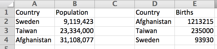
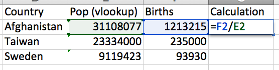
• In your spreadsheet, create two very simple tables on the same sheet, with an empty column between them. Give the first table the headings ‘Country’ and ‘Population’, and the second table the headings ‘Country’ and ‘Births’. We’re going to use VLOOKUP to grab the population from one table and put it next to the relevant country in the other.
• Type some names of countries in the relevant column in both tables. At least some of the countries should appear in both tables. It doesn’t matter what order they appear in – in fact, you’ll see the point of VLOOKUP best when the orders don’t match up.
• Type some numbers for the populations and births. The numbers don’t really matter for the purpose of this exercise – so type any you like.

Now normally these two tables would be much longer, and likely on separate worksheets – but starting this way makes it easier to see the process and avoid some early errors (which we’ll come onto later).

Before you write the VLOOKUP formula you need to decide which table, of the two, you want to bring the data into. You will write your formula in this table, and it will grab data from the other table.

We’ll choose the births one, for two reasons:

1. Firstly because our focus is going to be on births per person in a country
2. Secondly because there are more empty columns to the right of this one.

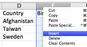
Right-click on the top of the column to the right of the one containing the data that is in both tables (in this case ‘Country’) and select ‘Insert’ to add a new column after that.

Call this column ‘Pop (vlookup)’.

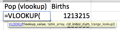
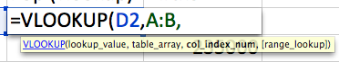
In the first cell of that new column, start typing the formula =VLOOKUP(. You’ll notice once you open the parenthesis, the tooltip appears telling you the ingredients this function needs.

Here’s a rough translation of what those ingredients mean:

• lookup_value means the value you are ‘looking up’ (in Google Sheets this is search_key)
• table_array means the range of cells (array) containing what you’re looking up and what you want to bring back (in Google Sheets this is range)
• col_index_num means the index number of the column with the values you you want to fetch back (in this case the populations). An index is a position like first, second, third, and so on – expressed as 1, 2, 3, and so on (in Google Sheets this is simply index)
• [range_lookup] – this is another optional ingredient, which basically asks whether you want the nearest match (in Google Sheets this is [is_sorted])

Put in plainer language, a VLOOKUP formula really means something like this:

=VLOOKUP(WHAT YOU ARE LOOKING FOR,WHERE YOU ARE LOOKING,WHICH COLUMN TO BRING BACK,NEAREST MATCH - TRUE OR FALSE)

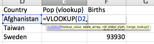
Let’s begin filling this formula up. Our first ingredient is what we are looking for. This is always the cell containing the value that should also be in the other table.

That’s our country, which is in cell D2. So our formula should now read:

=VLOOKUP(D2,

With a comma to end our first ingredient, we now enter the most important ingredient: the range of cells containing that and what we are looking for.

In this case, that’s columns A and B. The best way to do this is to select the range using your mouse by clicking and dragging across the two column letters. After typing a comma to end that ingredient, our formula reads like so:

=VLOOKUP(D2,A:B,

Our third ingredient is the index of the column we want to bring back. This will be a number, such as 1 for the first column in our range; 2 for the second and so on.

It’s important to remember that this index refers to the column in that range of cells. For example:

• In the column range A:C, index 3 is column C (the third column in that range)
• In the column range B:F, index 3 is column D (the third column in that range)

And so on.

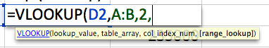
In our case, we want to bring back the value in the second column: the country’s population, so our formula needs to look like this:

=VLOOKUP(D2,A:B,2,

The final ingredient may be an optional one, but we do need to specify it.

This is whether we want this formula to grab the nearest match – TRUE or FALSE.

If you don’t specify either, Excel will assume you mean TRUE, and it will bring back the nearest match to your value.

In most cases, we don’t want this. If we’re looking for the population of Afghanistan, we don’t want Excel to bring back the population of Armenia.

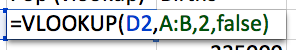
For that reason, type FALSE for this ingredient (it doesn’t have to be upper case), and close the parenthesis:

=VLOOKUP(D2,A:B,2,false)

This formula now means this:

=VLOOKUP(LOOK FOR THE VALUE IN D2,IN THE RANGE A:B,BRING BACK THE VALUE IN THE 2ND COLUMN IN THAT RANGE,BUT ONLY IF IT'S AN EXACT MATCH)

If your country in D2 was in column A in the other table, it should have brought back the population next to it.

If it wasn’t, then it should generate a #N/A error.

If you got that error, and didn’t expect it, check if you spelled the country exactly the same in both cells, including extra spaces. To check, copy from one and paste over the other.

Also check if the countries are in the first column in the range you specified (A:B in the example above)?

Once you’ve typed the formula once, you can obviously copy it down a whole column to look for each cell’s value in turn. When copied to cell E3, for example, the formula should read:

=VLOOKUP(D3,A:B,2,FALSE)

And in E4:

=VLOOKUP(D4,A:B,2,FALSE)

And so on.

This means you can now write a simple calculation to divide the births by population to get a birth rate per head (or times that by 1,000 to get a birth rate per thousand).

Using XLOOKUP

If you are using Google Sheets or a recent version of Excel you can use the XLOOKUP function to achieve the same results. This is a simplified version of VLOOKUP which removes the requirement to specify if you want the nearest match, and the requirement to specify a range containing both the matching column and the column you want to fetch data from (plus the index of the ‘fetch’ column).

An XLOOKUP formula has three ingredients:

• The cell or value you want to look up: this is called the lookup_value in Excel or search_key in Google Sheets
• The range of cells (i.e. the column) where there should be a match for that value: lookup_array in Excel or lookup_range in Google Sheets
• The corresponding range of cells (of the same length, i.e. another column) where the value you want to fetch should be: return_array in Excel or result_range in Google Sheets.

An XLOOKUP equivalent of our VLOOKUP formula, then, would look like this:

=XLOOKUP(D2,A:A,B:B)

Translated into a series of instructions this means:

LOOK FOR D2 IN COLUMN A, AND FETCH THE VALUE AT THE SAME POSITION IN column B

By asking you to specify the ‘matching’ (lookup) and ‘fetching’ (return/result) columns separately, it means they don’t have to appear in a certain order, and you don’t have to bother with an index.

Using a lookup formula on data in different sheets

One of the occasions where I used VLOOKUP was to bring together figures on charges for rape with figures on rape reports. These two sets of data were brought into the same workbook, but were clearly much bigger than the tables above, and occupied different sheets.

You can look for data in another sheet by adding the sheet name and an exclamation mark before the cell range like so:

'sheetname'!A:B

…replacing sheetname with the name of the sheet in question, but not forgetting to include the single quotation marks and exclamation mark.

In the rape data, for example, the sheet I wanted to pull data from was called ‘rape offences’, and so the formula looked like this:

=VLOOKUP(A6,'rape offences'!A:E,5,FALSE)

A6 contained the name of a police force. That police force, and around 40 others, were named in column A of the ‘rape offences’ sheet, and the data I wanted was in column E – so the range I was looking in had to be A:E, and the index 5.

Those pesky #N/A results

I mentioned above that if there is no match for what you are looking for, it will show #N/A. There are three possible reasons for this:

• There is no match at all. The name does not appear in that other table.
• There is no match in the first column of the range you specified. Perhaps you specified the wrong range of cells? Check.
• The name does appear in that column, but is typed slightly differently. For example, you may have ‘Devon and Cornwall’ in one table but ‘Devon & Cornwall’ in the other. That slight difference is enough to create a mismatch.

If you get a column full of #N/A, then it’s probably a problem with the range you’re looking in – or the data you’re looking in (or from) is consistently formatted with an extra space or other character which is leading to a mismatch (in Finding Stories In Spreadsheets I tackle some useful functions for stripping this out).

If you get some matches but there are lots of #N/A errors, you may need to re-evaluate your data. Perhaps you need another way to match. Names, for example, are often inconsistently used and entered. But codes tend to be much more consistent. If you have the option, use these to match separate sets of data.

Otherwise, even a small number of #N/A results is good news: it means you’ve got a much smaller manual workload than if you had to match all of them yourself.

You can now sort your data to bring those #N/A results to the top, and check each one manually.

For that manual process, try using the Find option under the Edit menu (or use the keyboard shortcut CTRL + F) to search yourself for what the formula was supposed to find.

If your value isn’t there at all, then no problem: the formula works: it should return an error if there’s no match (it may be that an organisation no longer exists).

If the value is slightly different, then try altering it manually so it matches, and see if the formula works when you return to the table containing it.

If you find yourself having to make the same sort of change more than once (such as removing a space, or changing an ampersand to the word ‘and’), then try some of the cleaning functions explained in Finding Stories In Spreadsheets.