
Sometimes an organisation will publish a spreadsheet where only a part of the full data is shown when you select from a drop-down menu. In order to get all the data, you’d have to manually select each option, and then copy the results into a new spreadsheet.
It’s not great.
In this post, I’ll explain some tricks for finding out exactly where the full data is hidden, and how to extract it without getting Repetitive Strain Injury. Here goes…
The example

To get the data from this spreadsheet you have to select 51 different options from a dropdown menu
The spreadsheet I’m using here is pretty straightforward: it’s a list of the populations for each fire and rescue authority in the UK (XLS). These figures are essential for putting any story about fires into context (giving us a per capita figure rather than just whole numbers) — and yet the authority behind the spreadsheet has made it very difficult to extract those numbers.
The population for each fire authority is on the second sheet of the workbook. The sheet defaults to figures for the population of England from 1971 to 2016 — to get the data for every authority in this spreadsheet you have to select another 50 different options from a dropdown menu, one by one.
There must be a better option.
Where is the data?

Select a cell with data and the formula bar will show a complex formula
The first step is to click on one of the cells containing the numbers you want — the numbers that change when a different option is selected from the drop-down menu.
When selected, look in the formula bar above the sheet (but below any menus) — highlighted with the red box in the image above.
The box will probably contain a formula that provides a clue to the location of the missing data. This one is quite a mouthful — but you don’t have to understand it to spot the name of a sheet which is not visible:
=IF(HLOOKUP($B$4,'rawdata and checks'!$B:$BB,A6-1969,FALSE)="..","..",ROUND(HLOOKUP($B$4,'rawdata and checks'!$B:$BB,A6-1969,FALSE),-2))
The formula is looking in a sheet called 'rawdata and checks' (the exclamation point is a useful clue to look for). That must be where the data is located. But this spreadsheet doesn’t have a sheet with that name — or at least one that we can see.
It must be hidden…
Find a hidden sheet in Excel
Instructions on how to hide a sheet in Excel — and, more importantly, how to unhide them — can be found in this Microsoft Office article.
In some instances that will be the end of the process. However, in this particular example the instructions don’t work — possibly because, as a note on that page explains:
“Note: If worksheets are hidden by Visual Basic for Applications (VBA) code that assigns the property xlSheetVeryHidden, you cannot use the Unhide command to display those hidden sheets. If you are using a workbook that contains VBA macros and you encounter problems when working with hidden worksheets, contact the owner of the workbook for more information.”
Alternatively, the hidden information may have been removed using the document inspector.
So we need a different approach…
Experiment with cell references to the hidden sheet
Let’s go back to the formula which is fetching the data from that hidden sheet. If that formula can fetch the data, then perhaps we can create more formulae which will cumulatively fetch all of it.
We could write a formula that grabs any specified cell from that sheet, like so (this is best done below the table so you have plenty of room):
='rawdata and checks'!A1
That cell is empty – but try copying it down one cell, so that it reads:
='rawdata and checks'!A2
This time the formula fetches a number: 1971. That’s the first year in the table above — a positive sign.
Now try copying the formula one to the right, so that it reads:
='rawdata and checks'!B1
The formula fetches ‘England’.
At this point you can start to copy these cells across and down until you have covered all the years, and all the countries — and the full dataset is there to be reused.
Another mystery: finding the hidden values for the drop-down list

Use the Data Validation option to see the values behind a drop-down list
In this example the values from the drop-down list are on the other sheet too — but what if they’re not?
To find the list that the drop-down menu is using you can look at various guides on how to create dependent drop-down lists, and reverse-engineer those. This is how to do it:
- Click on the cell which is being used for the drop-down list
- Select the *Data* menu, and then click on *Validation…* (or the *Data Validation* button)
- A *Data Validation* window should appear (shown above)
- On the default *Settings* view you should be able to see the Validation criteria. The third box on that view is *Source:*. This tells you which cells are being used to create a the drop-down list. In the Fire Service example above, that is `=$G$6:$G$56`
- Make a note of the cell range and exit the window by clicking **Cancel**.
- Look in the spreadsheet for those cells. It’s likely that they will have been hidden: if you can see the cells but not the values, try changing the text colour of those cells to black (they may have been made white to make them invisible). If you can’t see the cells, the column may have been hidden (see image below): in that case hover over the border between the two column letters until you get a two-lined double-arrow-headed cursor which allows you to click and drag to expand the hidden column.
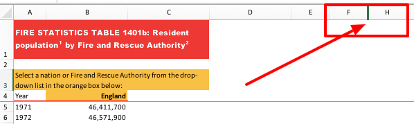
In this example column G is hidden – you can see that the columns skip from F to H
Once expanded, you should be able to see those hidden values being used by the drop-down.

PS: Data might also be shown in a chart but hidden from view. Instructions on that can be found here.
If you’ve found any other examples of data being hidden in spreadsheets, please let me know in the comments or on Twitter @paulbradshaw

Interesting
Reblogged this on MICHAEL OGAZIE.
Pingback: How to: uncover Excel data only revealed by a drop-down menu (Online Journalism Blog) | ResearchBuzz: Firehose
Pingback: Facebook, Google Sheets, Excel Sheest, More: Tuesday Afternoon Buzz, May 15, 2018 – ResearchBuzz
Pingback: How to uncover Excel data only revealed by a drop-down menu – Site Title
Reblogged this on Matthews' Blog.
I found a variation of this. Instead of using a normal column/row range, a named range from a hidden spreadsheet was used instead. I found it by first using the Home, Format, Hide & Unhide, Unhide Sheet. Then I was able to use Home, Find & Select, Go To to find the references to the named ranges.
thank you. This worked for me
this just saved me so much work thank you