

Treemaps are a great alternative to pie charts when you want to tell a story about the composition of something: whereas pie charts can be limiting, treemaps allow users to drill down into ‘parts of parts’, and group elements within particular categories.
In this post I’m going to show you how to create a treemap in the free visualisation software Tableau Public to show how the majority of BuzzFeed’s content views in 2015 took place away from its website.
This data suits a treemap particularly well: although the traffic is broadly split between ‘website’, ‘Facebook’, ‘Snapchat’, ‘YouTube’ and ‘other’, there are also subdivisions within some of those platforms – for example, Facebook traffic is split between video and images, and website traffic is split between direct visits, those via Google, and those via Facebook. A treemap allows users to explore those subtleties in a way that pie charts do not.
Step 1: Get the data in the right format
To create a treemap it is vital that you get the data in the correct format to begin with. In particular, you will need to make sure that as well as a primary ‘category’ column, you also have a second ‘sub category’ column. They don’t have to have these names, but that general concept is important. A third column should contain the values to be visualised.
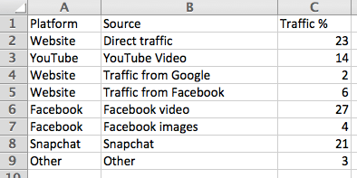
The key feature to look for in this data structure is that you should expect to see categories in your main ‘category’ column appear more than once. In our BuzzFeed data, for example, the platform category ‘website’ appears 3 times – once for each ‘Source’ sub category of ‘Direct traffic’, ‘Traffic from Google’ and ‘Traffic from Facebook’.
Also, make sure that your values only use numbers – don’t add percentage symbols, commas or other characters that might lead to it being interpreted as text and mean you have to reclassify the data later.
If you need a dataset to work with, I’ve uploaded the Buzzfeed figures here (you’ll need to save it to your computer).
Begin creating your chart
In Tableau Public, connect to the data you’ve just created, and go to your empty worksheet. On the left you should see your category (in this case, ‘Platform’) and sub category (in this case ‘Source’) columns in the Dimensions area; and underneath that in the Measures area, your values (in this case, ‘Traffic %’).
Click and drag your main category dimension (‘Platform’) into the Rows area at the top. Then do the same with your measure (‘Traffic %’) so that it looks like this:
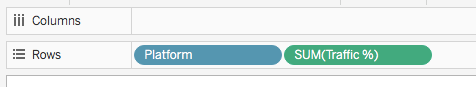
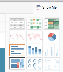
Tableau will automatically draw a chart for you – but ignore that. Instead, look to the right hand side where the ‘Show me’ menu should now be showing which chart types you can use with this combination of data. If it doesn’t show, click ‘Show me’ in the upper right corner.
One of the options available should be the treemap – it’s normally the first option four rows down. Click on this to change the chart to a treemap.
Now we have a treemap – but it’s only showing the top-level category (in this case, ‘Platform’). We need to customise it a bit to get a treemap which allows users to see the sub-categories too.
Customising the colours and slices
To the left of the chart itself you should see a box titled Marks containing buttons for Color, Size, Label, Detail and Tooltip. And underneath those buttons, icons indicating three settings:
- The ‘Size’ icon is set by ‘SUM(Traffic %)’
- The ‘Color’ icon is also set by ‘SUM(Traffic %)’
- The ‘Label’ icon is set by ‘Platform’

First we need to change it so that the ‘Color’ is determined by the main category (‘Platform’). To do that, click and drag the ‘Platform’ dimension onto the Color button.
Now, instead of one colour in different shades representing an amount, you should have five colours – one for each category:

We can customise the colour further by clicking on the ‘Color’ button and clicking Edit colors…. This will open up a new window with a list of categories on the left, and a palette on the right. In our case it makes sense to assign relevant colours to each platform: yellow for Snapchat, red for YouTube, and blue for Facebook. I’ve also chosen grey for ‘Other’. If you prefer other shades you can access other palettes using the dropdown menu in the upper right corner. Click ‘Apply’ to see the results, and ‘OK’ to apply and leave this window.

Next, we need to bring in that sub-category (‘Category’) in. A good place to do this is on the ‘Label’: because we are already using colour to indicate the platform, we need the label to add that extra information about the source of traffic to that platform.
To do this, click and drag the ‘Category’ dimension onto the Label button.
Now the area of colour for each platform should now split into further parts based on this new category. In addition, the text labels should reflect that information too.

Other customisation
The chart is now pretty much ready. That just leaves the title to customise: at the moment it is automatically taking the name of the sheet, so you can change the title by double-clicking on the sheet tab at the bottom and renaming it. Alternatively you can double-click on the sheet title and replacing it in the window that opens.
You can also customise the Tooltip – for example a % sign needs adding after the percentage figure on each slice.

Very helpful, many thanks for doing this.
When it comes to introducing the sub-category, you call it “sub-category (‘Category’)”. It might be more helpful to those going through step-by-step if you call it sub-category (‘Source’). Same with the ‘Category’ dimension a bit later on. Using the csv you provided it’s actually ‘Source’.